
A high-quality ADC preserves the nuances, dynamic contrasts, spatial cues, and harmonic textures that are essential for high-fidelity sound reproduction. It is particularly crucial in professional recording studios, where transparency and accuracy are non-negotiable for capturing master recordings. Furthermore, the ADC’s design influences the performance of digital filters, anti-aliasing strategies, and noise shaping techniques, all of which determine the integrity of the final signal. In essence, the ADC defines the initial boundary between the physical and digital domains, and its performance ultimately governs how faithfully a musical or sonic event is preserved for future listening, editing, and archival.
The process of PCM analog-to-digital recording is achieved in several steps, as detailed below:
Steps of ADC Operation
1. Sampling
- The analog signal is sampled at regular intervals. The sampling rate is determined by the Nyquist theorem, which states that the sampling frequency should be at least twice the highest frequency of the analog signal to avoid aliasing.
- Each sample is a snapshot of the signal’s amplitude at a specific moment.
2. Quantization
- The sampled signal is then quantized into discrete levels. The amplitude range of the analog signal is divided into a finite number of levels determined by the resolution of the ADC, typically measured in bits.
- For example, an 8-bit ADC divides the amplitude range into 28 =256 levels, while a 12-bit ADC divides it into 212 = 4,096 levels. For a 16 bit ADC 216 = 65,536 levels, and for a 24 bit ADC, 224 = 16,777,216 levels. A 32 bit ADC has 4,294,967,296 levels (-2,147,483,648 to +2,147,483,647 for signed 32-bit integers).
- Levels represent specific voltages. Silence, such as would be the case in between music tracks, is represented by 16 zeros for a 16 bit ADC, while the maximum loudness, where the peaks of the music waveform reach 0 dBFS, would be represented by 16 1’s. Any loudness (waveform peaks) higher than 0 dBFS would cause the signal to clip. At the crossover point in the waveform where the voltage is going from positive voltage to negative voltage, and is zero Volts, the 16 bits are also zeros.
- Since the levels represent specific (assigned) voltages, when music is encoded and a sample is taken, the nearest available integer level is assigned. It may not be the actual voltage that was in the signal path. The difference between what the voltage actually was, and the assigned voltage level, is called Quantization Error.
3. Encoding
- Each quantized level is assigned a unique binary code. This is the digital output corresponding to the input signal’s amplitude at a specific sampling instant.
Key Electrical Components and Processes
1 . Sample-and-Hold Circuit
- Captures and holds the analog signal’s voltage at each sampling instant. This ensures that the ADC processes a stable signal during quantization and encoding.
2 . Quantizer
- Converts the continuous voltage from the sample-and-hold circuit into one of the discrete levels. The accuracy of this process depends on the ADC’s resolution.
3 . Digital Encoder
- Converts the quantized level into a binary code, producing the digital output.
4 . Reference Voltage
- Determines the maximum and minimum amplitude range of the ADC. The signal is compared to this reference during quantization.
Types of ADC Architectures
1. Successive Approximation Register (SAR) ADC
- Uses a binary search algorithm to approximate the input signal step by step.
- Each step adjusts a digital-to-analog converter (DAC) to refine the approximation.
- Usually limited to less than 18-bits of resolution.
2. Flash ADC
- Employs a bank of comparators to simultaneously determine the quantization level, providing extremely fast conversion at the expense of complexity, resolution, linearity, and power consumption.
- Very good for video, radar, wideband radio receivers and other high speed applications that only require l4 to 10 bits of resolution.
3. Sigma-Delta ADC
- Oversamples the input signal and uses digital filtering and noise shaping to achieve high precision and near-perfect linearity. For a complete discussion about noise shaping, see An Audiophile’s Guide to Quantization Error, Dithering, and Noise Shaping in Digital Audio
4. Integrating ADC
- Measures the time taken for a ramp signal to match the input signal, providing high accuracy for low-speed applications.
ADC Mathematical Representation
The digital output D for a sampled input Vin is given by:
D = floor(Vin-Vmin/Vmax-Vmin x (2n-1))
Where:
- Vmin and Vmax are minimum and maximum reference voltages
- n = resolution of the ADC in bits
- 2n = the number of discrete levels (65,536 levels for a 16 bit ADC)
Key Considerations
- Resolution: Determines the smallest change in amplitude that the ADC can represent numerically.
- Sampling Rate: Affects the ability to accurately capture high-frequency signals.
- Signal-to-Noise Ratio (SNR): High resolution and precision help minimize noise and improve the digital representation.
- Linearity: The accuracy of the voltage step size between each numeric code. Linearity errors produce distortion.
By performing these processes electrically, an ADC enables analog signals, such as sound, temperature, or light intensity, to be processed by digital systems.

Modern Recordings Produced in 32-bit Resolution
Digital recordings are captured in 24-bit resolution but are typically mixed and mastered on 32-bit hardware. These systems can use 32-bit Integer or 32-bit Float.
Why 32-bit Recording Is Used:
1. Dynamic Range:
- 32-bit float recording provides an incredibly high dynamic range, which eliminates concerns about clipping or under-recording. It essentially means you cannot distort the audio by being too loud, as you can adjust the levels post-recording without losing quality.
2. Flexibility in Post-Processing:
- 32-bit float audio files allow engineers to recover seemingly “clipped” audio or amplify very quiet recordings without introducing noise.
3. Target Audience:
- 32-bit float recording is often aimed at professionals in film, television, and studio recording who demand ultimate flexibility and precision.
4. Modern Hardware Support:
- Devices like the Sound Devices MixPre series, Zoom F6, and some advanced DAWs support 32-bit float recording, making it increasingly accessible.
32-bit Integer vs. 32-bit Float:
- 32-bit integer offers extreme accuracy in representing digital signals but does not have the same kind of headroom as float. Each binary “word” is 32 bits in length (32 1’s and 0’s).
- 32-bit float offers the most dynamic range, so it allows for massive headroom and precision. The 32 bits are divided up into different functions (see below).
WAV files can have any sampling rate (integer value, not fractional).
- 8 bit is 0 to 255 with the zero crossing at 127
- 16 bit is +/- 32767 with zero crossing at 0 (+/-215)
- 24 bit is 2’s complement as there is no intrinsic 24 integer.
- 32 bit integer is +/- 2147483647 with zero crossing at 0 (+/-231)
- 32 bit integer and 32 bit floating point both require 4 bytes per sample. The IEEE Floating point standard seems to be what most people are using.
Is 32-bit Float Necessary?
For most everyday recording tasks, such as music production or podcasting, 24-bit is sufficient because it has 144 dB of dynamic range. However, for professional field recording or capturing unpredictable sound sources with a wide dynamic range, 32-bit float offers unmatched reliability. On the other hand, many recording engineers feel that 32-bit float is not necessary because even 24-bit covers more than the dynamic range of microphones.
Secrets Sponsor
Typical Microphone Dynamic Ranges:
1. Condenser Microphones:
- Dynamic Range: ~110–135 dB
- These microphones are known for their sensitivity and wide dynamic range, making them ideal for studio recordings of vocals and instruments.
- Example: A microphone with a self-noise of 15 dB(A) and a maximum SPL of 130 dB has a dynamic range of 115 dB.
2. Dynamic Microphones:
- Dynamic Range: ~90–120 dB
- These microphones are robust and handle high SPL well but may have a slightly narrower dynamic range compared to condensers. They’re commonly used for live sound and high-volume sources like drums or guitar amps.
3. Ribbon Microphones:
- Dynamic Range: ~90–115 dB
- Ribbon mics can have a slightly lower dynamic range due to higher self-noise, but modern active ribbon mics can offer improved performance.
Factors Affecting Dynamic Range:
- Self-Noise: The internal electronic noise of the microphone, typically measured in dB(A). Lower self-noise allows better capture of subtle details.
- Maximum SPL: The loudest sound the microphone can handle without distortion or damage. High maximum SPL is crucial for recording loud sources like drums or amplified guitars.
- Electronics and Design: High-quality preamps and circuitry in professional microphones enhance dynamic range.
Example Values:
- Neumann U87: Dynamic range ~117 dB (5 dB(A) self-noise, 122 dB maximum SPL).
- Shure SM7B: Dynamic range ~94 dB (low noise floor but with less sensitivity compared to condensers).
- Royer R-121 Ribbon Mic: Dynamic range ~90–95 dB.
Professional microphones often exceed the dynamic range of conventional audio interfaces and recording environments, but 32-bit sampling has a higher dynamic range than studio microphones.
Here is a Summary of Sampling and Dynamic Range:
The dynamic range of digital audio formats is determined by the bit depth, which defines the number of discrete amplitude levels that can be represented. Each additional bit increases the theoretical dynamic range by approximately 6 dB. Here’s how it breaks down:
1. 16-bit Audio
- Dynamic Range: ~96 dB
- Explanation: 6×16=96 dB
- Used in: CDs (Red Book standard), some broadcast formats.
- A 96 dB range is sufficient for most consumer playback environments but may be limiting for professional recording where very quiet or very loud sounds need to be captured without distortion or noise.
2. 24-bit Audio
- Dynamic Range: ~144 dB
- Explanation: 6×24=144 dB
- Used in: Professional recording and mixing, high-definition audio formats.
- A dynamic range of 144 dB exceeds the capabilities of most microphones, audio interfaces, and human hearing. It allows for a much lower noise floor and more headroom, making it ideal for professional use.
3. 32-bit Audio
- Dynamic Range: ~192 dB
- Explanation: 6×32=192 dB
- Used in: 32-bit floating-point formats for professional recording and production.
- Practical Notes:
- 32-bit Integer: Theoretical range is 192 dB, but it is rarely used because it far exceeds hardware capabilities.
- 32-bit Floating-Point: While still offering a theoretical 192 dB range, it is primarily valued for its practical benefits, such as preserving headroom and avoiding clipping in digital processing workflows. The dynamic range is effectively limited by the analog hardware.
Comparison with Human Hearing
- The dynamic range of human hearing is roughly 120 dB, from the threshold of hearing (~0 dB SPL) to the threshold of pain (~120 dB SPL). Thus:
- 16-bit audio captures most of what humans can perceive.
- 24-bit audio provides extra headroom for professional work and very quiet or loud sounds.
- 32-bit audio ensures no data loss in extreme scenarios like post- production processing or audio forensics.
So, higher bit depths offer greater dynamic range, but practical limitations like hardware and human perception make 24-bit audio the standard for professional-quality recording.
32-Bit Integer vs. 32-Bit Float Recording
Both 32-bit float and 32-bit integer recordings deal with digital audio, but they represent and process data differently. Here’s a breakdown of the key differences:
1. Representation of Audio Data
32-Bit Integer
- Uses 32 bits to represent each sample as a fixed-point integer.
- Values are represented within a specific range (e.g., -2,147,483,648 to 2,147,483,647 for signed 32-bit integers).
- Offers high precision but operates within a fixed dynamic range.
32-Bit Float
- Uses 32 bits to represent audio data in a floating-point format:
- 1 bit for the sign (positive or negative).
- 8 bits for the exponent (dynamic range control).
- 23 bits for the mantissa (precision).
- Offers a dynamic range so large that clipping becomes nearly impossible.
- Provides a theoretical dynamic range of 1,528 dB, far beyond human hearing.
- Prevents audible quantization errors for fades, reverb tails, etc.
- There is no loss in resolution to represent low amplitude signals.
2. Dynamic Range
32-Bit Integer
- Fixed dynamic range based on the bit depth.
- For 32-bit integer audio, the dynamic range is about 192 dB.
32-Bit Float
- Floating-point arithmetic enables an essentially infinite headroom during recording.
- Allows signals far above 0 dBFS (Full Scale) to be recorded without distortion.
3. Use Cases
32-Bit Integer
- Common in mastering and production workflows where high precision is necessary for audio processing.
- Suitable for studio recordings, where levels are controlled.
32-Bit Float
- Ideal for field recording or situations with unpredictable audio levels (e.g., live events, nature recordings).
- Allows adjustment of levels after recording without introducing noise or distortion.
4. Clipping and Noise Floor
32-Bit Integer
- If audio exceeds 0 dBFS, it clips, and the distortion is permanent.
- Very quiet signals can still be recorded accurately but boosting them too much may introduce noise.
32-Bit Float
- Cannot clip in the recording stage because signals exceeding 0 dBFS are stored without distortion and can be scaled back down in post-production.
- Quiet signals can be amplified without raising the noise floor.
5. File Size and Performance
32-Bit Integer
- Files are smaller compared to 32-bit float because they don’t need to store exponent information.
- Requires less processing power than 32-bit float.
32-Bit Float
- Files are slightly larger because they store more information (mantissa and exponent).
- Processing is more complex but manageable with modern hardware.
6. Hardware and Software Support
32-Bit Integer
- Supported by most professional digital audio workstations (DAWs) and hardware.
32-Bit Float
- Supported by high-end recorders (e.g., Zoom F6, Sound Devices MixPre series) and many modern DAWs.
- Ideal for workflows where audio fidelity and post-production flexibility are paramount.
Summary
| Feature | 32-Bit Integer | 32-Bit Float |
| Dynamic Range | ~192 dB | ~1,528 dB |
| Headroom | Fixed | Virtually unlimited |
| Clipping | Can clip | Cannot clip |
| File Size | Smaller | Slightly larger |
| Use Cases | Controlled recording | Unpredictable recording |
| Hardware Support | Universal | Limited but growing |
For most controlled studio recordings, 32-bit integer is sufficient. For field recording or unpredictable audio environments, 32-bit float is a game-changer. But, as I said, 32-bit float is still in development and testing.
Secrets Sponsor
Commercial 32-bit ADCs
There are several commercial analog-to-digital converters (ADCs) capable of 32-bit encoding, primarily designed for high-performance audio applications. Here are some notable examples:
Texas Instruments PCM1820
A stereo-channel, 32-bit, 192-kHz audio ADC with a 113-dB signal-to-noise ratio (SNR).
Texas Instruments PCM1841-Q1
An automotive-grade, quad-channel, 32-bit, 192-kHz audio ADC.
Asahi Kasei Microdevices (AKM) AK5558VN
An 8-channel, 32-bit, 768-kHz premium ADC achieving a 115-dB dynamic range, suitable for mixers and multi-channel recorders.
Analog Devices LTC2508-32
A low-noise, low-power, high-performance 32-bit ADC with an integrated configurable digital filter, operating from a single 2.5V supply.
Asahi Kasei Microdevices (AKM) AK5538VN
An 8-channel, 32-bit, 768-kHz advanced audio ADC achieving a 111-dB dynamic range, suitable for digital audio systems.
These ADCs are utilized in professional audio equipment, high-fidelity recording systems, and other applications requiring exceptional audio quality.
32-bit Float is Performed by DAW (Digital Audio Workstation) Software Rather than an ADC.
The creation of 32-bit floating-point audio depends on the specific context and is typically handled by DAW software rather than directly by the ADC. Here’s a breakdown:
1. Role of the ADC (Analog-to-Digital Converter):
- Bit Depth of ADC: Most ADCs in professional audio interfaces operate at a maximum of 24-bit fixed-point resolution. This is the physical limitation of the hardware, as ADCs convert analog signals into a fixed number of digital levels.
- Dynamic Range: High-quality ADCs achieve a dynamic range close to 144 dB, matching the theoretical limit of 24-bit fixed-point audio.
No ADC natively produces 32-bit floating-point audio because the floating-point format is unnecessary for the ADC’s task of converting analog voltages into discrete digital levels. Instead, 32-bit floating-point is used later in the digital domain.
2. Role of the DAW and Software:
- 32-bit Floating-Point Conversion: Most DAWs or audio software convert the 24-bit fixed-point output from the ADC into 32-bit floating-point format. This conversion is done to facilitate high-resolution internal processing, avoid clipping, and improve headroom during mixing and editing.
- Advantages in the DAW:
- Prevents rounding errors during complex operations (e.g., summing, gain changes, and effects).
- Avoids clipping when signals exceed 0 dBFS during processing, as the floating-point format can represent values beyond the fixed-point ceiling.
- Ensures precision when working with very low-level signals.
3. Special Cases: 32-bit Float ADC Interfaces
- Some modern audio interfaces claim to record in 32-bit floating-point natively. However:
- The actual ADC conversion still happens at 24-bit fixed-point (the hardware standard).
- A DSP stage inside the interface (before the signal is sent to the DAW) converts the 24-bit fixed-point signal to 32-bit floating-point.
- The primary purpose is to preserve the extended headroom and avoid clipping during the conversion process, particularly in scenarios where input gain is not set optimally.
Summary
- ADC Output: Typically 24-bit fixed-point.
- 32-Bit Float Creation: Performed by DAW software or, in some cases, a DSP stage in an audio interface.
- Why 32-Bit Float? To enhance processing precision, prevent clipping, and provide an extensive dynamic range for mixing and editing in the digital domain.
While 32-bit floating-point audio offers benefits in the production pipeline, it generally exceeds the capabilities of most playback systems and human hearing, making it unnecessary for final distribution.
Costs of 32-bit Integer ADCs
The cost of commercial 32-bit ADCs varies significantly depending on the brand, features, and intended application. Here’s a breakdown of factors affecting their cost and some general price ranges:
1. Price Ranges
- Entry-Level Models: Some 32-bit ADCs (the chips) with basic features (low channel count, moderate sampling rates) might cost around $5–$20 per unit in bulk for applications like embedded systems or automotive audio.
- Mid-Range Models: 32-bit ADCs designed for high-quality audio (e.g., for professional recording or audiophile equipment) typically cost between $20–$100 per unit.
- High-End Models: High-performance ADCs with multiple channels, very high sampling rates, or specialized features (like built-in filters or ultra-low noise) can cost $100–$500+ per unit or more, especially in lower quantities.
2. Key Factors Influencing Cost
- Performance Specifications:
- Higher dynamic range and lower noise increase costs.
- Support for ultra-high sampling rates (e.g., 768 kHz) also adds to the price.
- Channel Count:
- Single-channel ADCs are cheaper.
- Multi-channel ADCs (e.g., 8-channel or higher) cost more due to increased complexity.
- Additional Features:
- Integrated digital filters, programmable gain, or DSP capabilities raise prices.
- Automotive-grade or ruggedized components for industrial use are more expensive.
- Volume:
- Prices drop significantly when purchased in bulk (thousands of units) compared to small orders.
- Brand and Support:
- Premium brands like Analog Devices, Texas Instruments, or Asahi Kasei Microdevices (AKM) often charge a premium for their reputation and extensive technical support.
While 32-bit ADCs can be relatively costly compared to 16-bit or 24-bit models, they aren’t prohibitively expensive for industries or professionals who require their precision and dynamic range. For audiophile or professional-grade equipment, the added cost is often justified by the improved audio quality.
DACs Converting Digital Back to Analog
In essence, Digital-to-Analog Converters (DACs) and Analog-to-Digital Converters (ADCs) are opposite processes, but DACs don’t strictly “reverse” the procedure used by ADCs. Here’s why:
ADC Process (Analog to Digital Conversion)
- Sampling: The analog signal is sampled at regular intervals (defined by the sampling rate, e.g., 44.1 kHz, 96 kHz, or 192 kHz).
- Quantization: Each sample is assigned a discrete value based on the bit depth (e.g., 16-bit, 24-bit, or 32-bit), representing the amplitude of the signal at that point.
- Encoding: The quantized values are stored or transmitted as a digital binary sequence.
DAC Process (Digital to Analog Conversion)
- Interpolation and Reconstruction: The DAC processes the digital samples and converts them into a smooth, continuous waveform. This often involves oversampling and filtering to reconstruct the original signal as closely as possible.
- Conversion to Voltage: The digital binary data is converted into corresponding voltage levels.
- Filtering: A low-pass filter removes high-frequency artifacts (e.g., aliasing or staircase effects) introduced during the conversion, ensuring a smooth analog signal.
A PCM (Pulse Code Modulation) DAC (Digital-to-Analog Converter) knows where a 24-bit sample begins and ends based on the format and clocking of the digital audio data it receives. The process depends on the digital audio interface being used. Here’s how it works:
1. Serial Data Transmission & Bit Clock
- PCM audio data is typically transmitted serially (bit by bit) rather than in parallel.
- A Bit Clock (BCLK) governs the timing of each bit, ensuring the DAC reads the data at the correct rate.
2. Frame Sync (Word Clock)
- A Word Clock (or Frame Sync, LRCLK) signal defines the boundaries of each audio sample.
- In I2S (Inter-IC Sound) format, for example:
- The Left-Right Clock (LRCLK) changes state at the start of each sample.
- The transition from low to high (or vice versa) signals that a new sample is starting.
- This indicates whether the current data belongs to the left or right channel.
3. Bit Depth Awareness
- The DAC must be configured to expect a specific word length (e.g., 16-bit, 24-bit, 32-bit).
- For a 24-bit sample in a 32-bit frame, the DAC may either:
- Read the 24 most significant bits (MSBs) and ignore the least significant bits (LSBs).
- Expect the data to be left-justified or right-justified, depending on the format.
4. Common Digital Audio Formats & Sample Framing
- I2S (Inter-IC Sound)
- LRCLK toggles for each sample.
- Data is left-aligned, starting after one BCLK delay.
- TDM (Time-Division Multiplexing)
- A frame sync pulse marks the start of a new data frame containing multiple channels.
- Right-Justified / Left-Justified PCM
- Determines whether the sample data is aligned to the start or end of the word clock frame.
5. Synchronization with Master Clock (MCLK)
- Some DACs use a separate Master Clock (MCLK) to synchronize the internal processing of data.
- The DAC may derive timing from this or use it for oversampling and interpolation.
Summary
A PCM DAC determines where a 24-bit sample starts and ends by using the word clock (LRCLK), the bit clock (BCLK), and the known data format. These signals ensure that each sample is correctly framed, transmitted, and converted to an analog signal accurately.
Key Differences Between ADC and DAC
1. Direction:
- ADC converts a continuous analog signal into a discrete digital format.
- DAC converts discrete digital data back into a continuous analog signal.
2. Process Complexity:
- ADCs need to account for anti-aliasing by applying a low-pass filter before sampling to avoid high-frequency noise folding into the sampled signal.
- DACs focus on reconstructing the smooth analog signal by using interpolation and low-pass filtering.
3. Irreversibility:
- Some information might be lost during the ADC process due to quantization error (rounding errors during sampling). DACs cannot “recover” this lost data.
- Noise or distortion introduced during digital encoding or storage may further affect the output quality.
4. Mathematical Models:
- ADCs rely on algorithms for sampling and quantization (Nyquist-Shannon theorem applies).
- DACs often use interpolation techniques like zero-order hold or higher- order filters to reconstruct the waveform.
Summary
While DACs aim to reconstruct the original analog signal as closely as possible, they don’t strictly “reverse” the ADC process because:
- Some information lost during ADC cannot be recovered.
- DACs use their own methods, like oversampling and interpolation, to create a continuous analog waveform.
The two are complementary, but their operations are tailored to their respective directions of conversion.
What About the Distribution Format of 32-bit Studio Recording Masters?
32-bit studio recording files are typically down-converted (down-sampled) to 24- bit or 16-bit files for distribution. Here’s why and how this process works:
Why Down-Convert (Down-Sample)?
1. Compatibility:
- Most consumer playback systems and formats (CDs, streaming services, etc.) do not support 32-bit audio. Standard distribution formats include:
- 16-bit/44.1 kHz for CDs.
- 24-bit/48-96 kHz for high-resolution formats like FLAC or WAV.
- 32-bit files are primarily used during recording and production stages, not playback.
2. File Size:
- 32-bit files are significantly larger than 16-bit or 24-bit files, which would make them impractical for distribution to consumers. Such formats would certainly be impractical on streaming services.
3. Audibility:
- The human ear cannot perceive the extra dynamic range provided by 32- bit files. A 24-bit file already provides a theoretical dynamic range of 144 dB, which far exceeds what humans can hear (~120 dB).
4. Standardization:
- Industry standards like CDs and streaming platforms require specific bit depths and sample rates for distribution.
How the Down-Conversion Works
1. Dithering:
- When reducing bit depth from 32-bit to 24-bit or 16-bit, dithering is applied. Dithering adds a small amount of noise to mask quantization errors and prevent audible artifacts caused by the reduction in bit depth.
2. Noise Shaping (Optional):
- In some cases, noise shaping is used during dithering to push noise to less perceptible frequencies, improving the perceived quality of the audio.
3. Sample Rate Conversion (if needed):
- If the original recording is at a high sample rate (e.g., 96 kHz or 192 kHz), it may also be down-sampled to 44.1 kHz (CD) or 48 kHz (streaming) to meet distribution requirements.
What Exactly is Dithering?
Dithering in digital audio down-conversion is a process used to minimize audible artifacts and distortion caused by quantization errors when reducing the bit depth of a digital audio file (e.g., from 24-bit to 16-bit). Here’s a breakdown of what dithering entails:
1. Understanding Quantization Error
- Quantization: When reducing bit depth, the digital system must approximate each sample’s amplitude to the nearest level available at the new bit depth.
- Error: This rounding introduces quantization noise, which can manifest as distortion or artifacts, especially in low-level signals.
2. What Dithering Does
Dithering involves adding a small amount of random noise to the signal before reducing its bit depth. This noise “smooths out” quantization errors by randomizing their impact, preventing the errors from creating noticeable distortion or patterns in the audio.
3. How It Works
- Adding Noise: A low-level, pseudo-random noise signal is added to the original digital audio signal.
- Bit Depth Reduction: The signal is quantized to the new bit depth (e.g., 16-bit), including the added noise.
- Perceptual Effect: The added noise masks quantization artifacts, spreading the distortion energy across a broad frequency range. The result is a cleaner and more natural sound.
4. Benefits of Dithering
- Reduces Harmonic Distortion: Dithering turns quantization distortion into a more uniform, low-level noise that is less perceptible to the human ear.
- Improves Low-Level Detail: In quiet passages or low-level signals, dithering ensures that subtle details are preserved, making the audio sound more natural.
- Prevents Repetitive Patterns: Without dithering, quantization errors can produce audible and undesirable periodic patterns, especially in tonal music.
5. Types of Dithering
- White Noise Dithering: Adds unshaped random noise. This is simple but not optimal for all use cases.
- Noise Shaping Dithering: Adds noise with a frequency spectrum tailored to human hearing, pushing noise energy into less perceptible frequency ranges (e.g., ultrasonic frequencies).
- Triangular Probability Density Function (TPDF) Dithering: A common and effective method where the noise distribution is triangular rather than Gaussian.
6. When Is Dithering Used?
- During bit depth reduction, such as converting 24-bit recordings to 16-bit for CD production.
- In mixing and mastering, to preserve sound quality during final exports.
- When combining or bouncing tracks with different bit depths.
7. Drawbacks
- Adds Noise: While the added noise is low-level and typically imperceptible, it still increases the overall noise floor slightly.
- Irreversible: Once dithered, the noise becomes part of the audio signal and cannot be removed.
Summary
Dithering is a critical process in digital audio production that helps maintain sound quality when reducing bit depth. By adding carefully controlled random noise, it mitigates the harsh effects of quantization errors, resulting in a smoother and more natural audio experience.
Distribution Formats
1. 16-Bit (CD-Quality):
- Used for CDs and some streaming services.
- Standardized at 16-bit/44.1 kHz.
2. 24-Bit (High-Resolution Audio):
- Used for audiophile-grade formats like FLAC, ALAC, and WAV.
- Typical sample rates range from 48 kHz to 192 kHz. Some streaming services offer “High-Rez” subscriptions for this.
When 32-Bit Files Are Retained
- Archiving:
- Studios often archive the original 32-bit float or integer recordings for future use, such as remastering or re-editing.
- Professional Workflows:
- Producers and engineers may retain 32-bit files during the mixing and mastering stages to avoid data loss during processing.
In Summary
- While 32-bit recording offers immense flexibility and quality during production, it is not practical or necessary for distribution. Files are down-converted to 24-bit or 16-bit formats with proper dithering to ensure they are compatible with playback devices and streaming services and are optimized for human hearing.
What are the Mathematics of Down-Converting 32-bit to 24-bit Audio?
The process of down-converting 32-bit audio to 24-bit audio involves mathematical operations to reduce the bit depth while preserving audio quality. Here’s a detailed breakdown of the mathematics and concepts behind this process:
1. Understanding Bit Depth
- 32-bit float audio represents sound using floating-point numbers:
- 1 sign bit, 8 exponent bits, and 23 mantissa bits.
- Provides a huge dynamic range (~1,528 dB) and prevents clipping.
- 24-bit audio uses fixed-point integers with values ranging from 223 to 223 – 1, providing a dynamic range of ~144 dB.:
When converting from 32-bit float to 24-bit integer:
- The floating-point values are scaled to fit within the fixed-point range.
- Quantization is applied to round the data to discrete integer values.
2. Steps in Down-Conversion
Step 1: Scaling the Audio Values
32-bit float audio stores samples in a normalized range:
- Values typically range between −1.0 and 1.0.
To convert to 24-bit integer:
- Scale the floating-point values to fit the 24-bit integer range [−8,388,608,8,388,607]
- Formula: y24-bit = round(Xfloat x 8,388,608), where:
- Xfloat is the normalized 32-bit float sample.
- y24-bit is the resulting 24-bit integer sample.
Step 2: Quantization
Quantization occurs as part of scaling, where:
- Decimal values are rounded to the nearest integer within the 24-bit range.
- This step introduces quantization error, which can create subtle distortions in the audio signal.
Step 3: Dithering
To reduce audible artifacts caused by quantization error:
- Dithering adds low-level random noise to the signal before quantization.
- This masks the quantization noise, making it less perceptible.
The dithering noise is statistically distributed and typically shaped to emphasize frequencies less noticeable to human ears (e.g., high frequencies).
Step 4: Clipping Prevention
If the original 32-bit float signal exceeds the range −1.0-1.0−1.0 to 1.01.01.0:
- These samples are clipped to the maximum/minimum values of the 24-bit integer range.
Formula for clipping:

3. Noise and Distortion
- Quantization Noise: Results from mapping continuous values to discrete levels.
- Dithering Noise: Intentionally added to randomize quantization error.
The signal-to-noise ratio (SNR) for a 24-bit system is about 144 dB, meaning that the quantization noise is effectively inaudible for most practical purposes.
4. Practical Considerations
- Normalization: Ensure that the audio does not exceed the maximum range after conversion.
- Bit Truncation: If the audio is stored as 32-bit integer instead of float, down- conversion may involve truncating the least significant bits directly.
- For example, taking only the 24 most significant bits: y24-bit = [x32-bit /256]
Summary of Key Equations
1. Scaling:
y24-bit = round(Xfloat x 8,388,608)
2. Dithering (Random Noise):
Xdithered = Xfloat + ndither
Where ndither is low-level random noise.
3. Clipping:
Yclipped = min(max(y24-bit , – 8,388,608), 8,388,607))
By following these mathematical operations, a high-quality 24-bit audio file is generated from a 32-bit source, preserving as much detail and fidelity as possible.
What is DXD Digital Recording?
DXD, or Digital eXtreme Definition, is a high-resolution digital audio recording format initially developed for editing recordings made in the DSD (Direct Stream Digital) format used by SACD (Super Audio CD). DXD provides a way to work with audio in a more flexible and accurate domain compared to DSD, which is less editable due to its 1-bit structure.
Key Features of DXD
- High Sampling Rate: DXD uses a sampling rate of 352.8 kHz (or 384 kHz in some cases) at 24-bit resolution, which is significantly higher than the standard 44.1 kHz or 48 kHz used in CD-quality recordings.
- Bit Depth: The format uses a 24-bit resolution, which allows for a high dynamic range and minimizes quantization noise.
- PCM Format: DXD is a type of PCM (Pulse Code Modulation) format, offering greater flexibility for editing, mixing, and processing audio compared to the 1-bit DSD format.
- Designed for DSD Workflow:
- Audio recorded in DSD can be converted to DXD for editing and processing because DSD is challenging to edit directly.
- After editing in DXD, the audio can be converted back to DSD for final output or distribution.
Advantages of DXD
- Precision in Editing: The high sampling rate and bit depth allow engineers to make precise edits and apply effects with minimal degradation of audio quality.
- Flexibility: Unlike DSD, DXD supports advanced digital audio processing techniques.
- High Fidelity: The extremely high resolution ensures that audio retains its natural sound even after multiple stages of processing.
Use Cases
- Professional Audio Production: Especially in classical, jazz, and audiophile-grade recordings where pristine audio quality is a priority.
- Hybrid SACD Production: DXD is often used in the workflow for creating SACDs.
- Mastering and Mixing: Engineers use DXD for its balance of editability and high-quality audio fidelity.
DXD has become one of the standards in high-end audio recording and production, particularly for projects aimed at audiophile audiences.
When a Digital Music File is Played, a Digital Low-Pass Filter is Applied to Prevent Aliasing
When a digital music file is played, a low-pass filter – commonly called a reconstruction or anti-imaging filter – is essential for converting the discrete digital samples back into a continuous analog waveform. It is applied during playback, not when it is recorded. This filter removes ultrasonic images produced during digital-to-analog conversion, which result from the discrete-time sampling process. Without it, these high-frequency artifacts could alias into the audible range or generate intermodulation distortion in downstream analog components.
The design and behavior of this low-pass filter depend heavily on the sampling rate of the digital file. For 16-bit/44.1 kHz audio (CD quality), the filter must sharply attenuate frequencies above 22.05 kHz, which demands a steep transition band and can introduce time-domain artifacts such as pre-ringing. At higher sample rates – like 24-bit/96 kHz or 24-bit/192 kHz – the Nyquist frequency increases to 48 kHz and 96 kHz respectively, allowing for a much wider transition band.
This gives filter designers more freedom to implement gentler slopes, minimum-phase designs, or even analog-style slow roll-off characteristics that preserve transient response and reduce ringing. As a result, playback of high-resolution files often sounds more natural and open, not just because of greater bit depth or frequency range, but due to improved filtering. The low-pass filter thus plays a pivotal role in audio fidelity, and its implementation must be carefully tailored to the sample rate to balance frequency accuracy with time-domain clarity. In short, it is the final gateway through which digital audio becomes music again, and its importance cannot be overstated.
A low-pass filter is also necessary with DSD (Direct Stream Digital) sampling – arguably even more so than with PCM. While DSD uses a very high sampling rate (typically 2.8224 MHz for DSD64), it relies on 1-bit sigma-delta modulation and noise shaping to push quantization noise into ultrasonic frequencies well above the audible range.
This design produces an analog-like waveform that can be smoothed with a simple analog low-pass filter, but the key issue is that the ultrasonic noise floor is very high, especially above 50 kHz. If left unfiltered, this high-frequency energy can cause intermodulation distortion in amplifiers and tweeters, which are not designed to handle significant energy at those frequencies.
Unlike PCM, where steep digital filters can be implemented prior to the DAC stage, DSD typically minimizes digital filtering to preserve timing and transient response. Instead, it relies on a gentle analog low-pass filter after the DAC to remove ultrasonic noise while keeping the time-domain integrity of the signal. For DSD64, a low-pass cutoff around 50–100 kHz is typical. Higher-rate DSD variants like DSD128 or DSD256 allow even more relaxed filtering, which improves fidelity but still requires filtering to protect playback hardware.
The impulse response shape of a low-pass filter used for anti-aliasing and reconstruction in PCM sampling depends on the type of roll-off characteristic applied. There are three common types:
1. Sharp (Brickwall) Roll-Off
- Impulse Response Shape: A long sinc function (see below for a definition of the sinc function).
- Characteristics:
- Nearly perfect frequency response with a flat passband and a steep cutoff.
- Exhibits significant time-domain ringing due to the sinc function extending infinitely in both directions.
- Pre-ringing and post-ringing can be audible, affecting transient response.
2. Slow (Gradual) Roll-Off
- Impulse Response Shape: A tapered sinc function with a shorter duration.
- Characteristics:
- Less steep frequency roll-off, allowing some aliasing.
- Reduces time-domain ringing compared to sharp filters.
- Improves transient response by minimizing pre-ringing artifacts.
3. Minimum Phase Roll-Off
- Impulse Response Shape: Asymmetric, with energy concentrated after the main impulse.
- Characteristics:
- Eliminates pre-ringing, which is often perceived as unnatural.
- Has a faster response to transients, leading to a more natural sound.
- More phase distortion compared to linear-phase filters.
Each of these roll-off types has trade-offs between frequency accuracy, transient response, and ringing artifacts. The choice depends on the application, with sharp roll-off used in precision audio applications, slow roll-off for a balance between aliasing and time-domain response, and minimum-phase roll-off preferred for psychoacoustic optimization.
Here are impulse response simulation spectra for the three types of roll-off filters. Pre-ringing occurs at -0.10 to -0.02 seconds before the main signal at 0 seconds, and post-ringing occurs at +0.02 to +0.10 seconds.
![]()
![]()
![]()
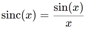
Definition of the Sinc Function:
The sinc function is defined as:
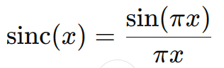
Where:
x represents the time-domain variable. The function has a central peak at x = 0 and oscillates with decreasing amplitude as x moves away from zero. This is what is called the normalized sinc function. This form is widely used in signal processing and Fourier analysis because it leads to nice properties, like the Fourier transform of a rectangular pulse being a sinc function.
However, there’s also an unnormalized version often used in pure mathematics:
The Sinc Function Role in Low-Pass Filters and Impulse Responses:
Ideal Low-Pass Filter Impulse Response:
- The sinc function represents the impulse response of an ideal brickwall low-pass filter in the time domain.
- A perfect low-pass filter that cuts off all frequencies above a certain threshold has an impulse response that extends infinitely in both directions as a sinc function.
- Why It Causes Ringing:
- Because the sinc function extends infinitely in both directions, any signal filtered by it will have pre-ringing and post-ringing artifacts (oscillations before and after a transient).
- The sharp frequency cut-off leads to Gibbs phenomenon, causing overshoot and ringing in the time domain.Windowed Sinc Filters:
- Real-world implementations truncate the sinc function using windowing techniques to make it finite in length.
- Windowed sinc filters, such as those using a Hann, Hamming, or Blackman window, reduce ringing but also slightly compromise frequency response.
How It Relates to Digital Audio:
- Sharp Roll-Off Filters use a longer sinc function, preserving frequency accuracy but causing more time-domain ringing.
- Slow Roll-Off Filters use a shorter sinc function to reduce ringing but allow some aliasing.
- Minimum Phase Filters modify the sinc function asymmetrically to remove pre-ringing, improving transient response.
The sinc function is fundamental in reconstructing audio from digital samples, ensuring that the signal remains accurate while balancing frequency precision and time-domain artifacts.
Analog audio circuits do not produce pre-ringing in the same way that digital audio circuits do. Pre-ringing is a phenomenon primarily associated with digital signal processing, particularly in linear-phase digital filters and certain types of oversampling or reconstruction filters.
Why Digital Circuits Exhibit Pre-Ringing:
- Filtering and Impulse Response: In digital audio, linear-phase FIR (Finite Impulse Response) filters introduce symmetrical ringing before and after a transient due to their impulse response. This is a mathematical consequence of how these filters maintain phase linearity.
- Upsampling and Interpolation: Many digital-to-analog converters (DACs) use oversampling and interpolation filters that can introduce pre-ringing artifacts.
- Windowing Effects: When applying certain digital signal processing techniques like windowing or Fourier transforms, artifacts resembling pre-ringing can occur.
Why Analog Circuits Avoid Pre-Ringing:
- Minimum-Phase Behavior: Most analog filters are minimum-phase, meaning their impulse response is asymmetrical and does not create pre-ringing. Instead, any ringing they introduce occurs after the transient, known as post-ringing.
- Lack of FIR Filtering: Analog filters are typically implemented using reactive components (resistors, capacitors, and inductors), which behave differently from FIR filters in digital systems.
- Natural Response: Analog systems often have gradual roll-offs and natural decay characteristics that avoid the sharp transitions responsible for digital pre-ringing.
Analog circuits may introduce post-ringing or resonance depending on their design (e.g., high-Q filters or transformers), but they do not exhibit the unnatural pre-ringing artifacts found in digital processing.
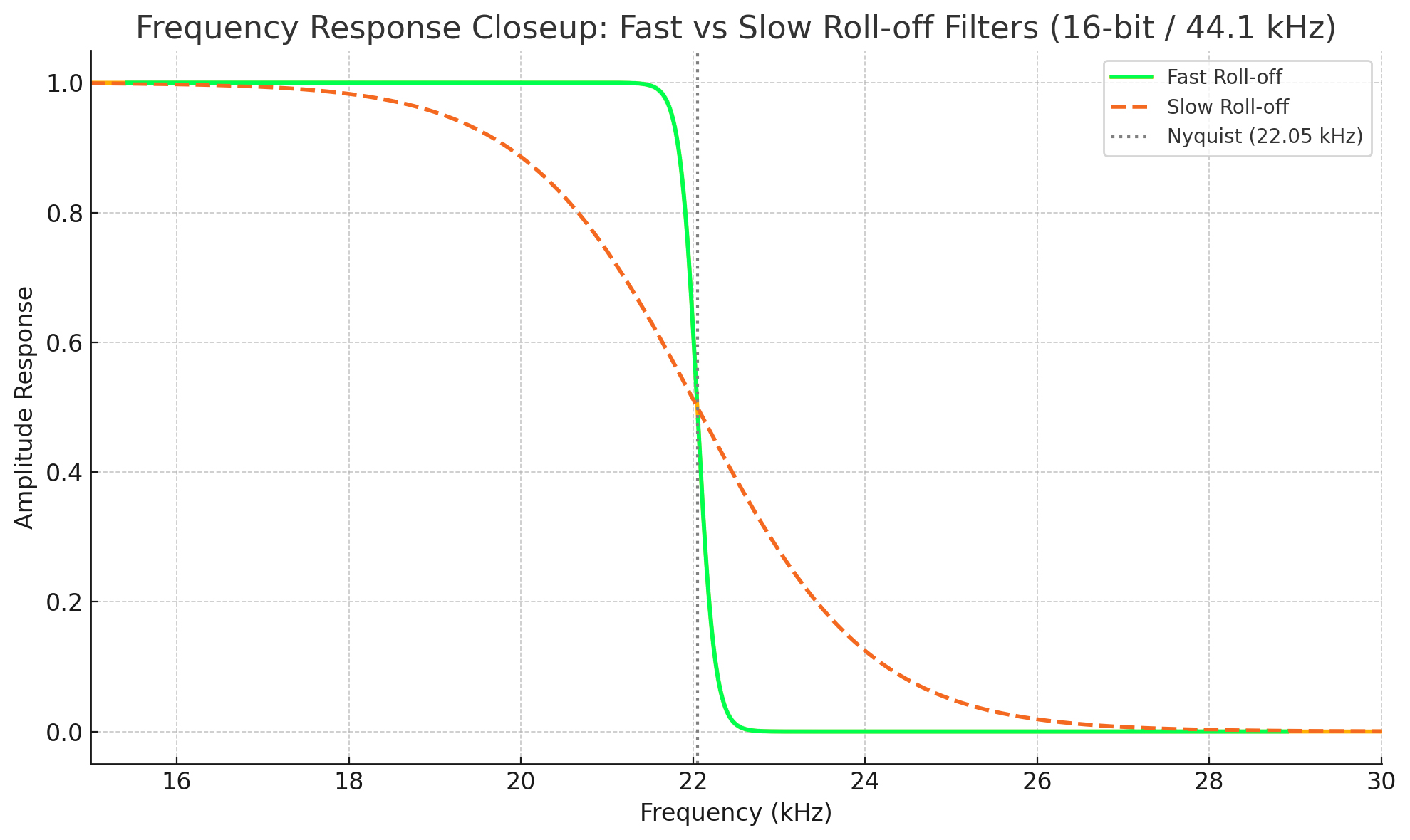
Here is a frequency response plot of a fast roll-off low-pass filter and slow roll-off low-pass filter with 16/44.1 sampling, zoomed in at the roll-off point. You can see that the fast roll-off begins at about 21.5 kHz and ends at 22.5 kHz, while the slow roll-off begins at about 16 kHz and ends at 28 kHz.
Note that the roll-off rate of a filter – how quickly it attenuates frequencies beyond the cutoff – is not determined by whether it’s minimum phase or slow roll-off, because these describe different aspects of the filter:
Minimum Phase vs. Slow Roll-off:
- Minimum phase refers to the phase characteristics of a filter. A minimum phase filter has the least possible phase shift for a given magnitude response. It typically has faster time-domain response (less pre-ringing), which is useful in audio and other real-time applications.
- Slow roll-off refers to the steepness of the filter’s frequency cutoff. A slow roll-off filter gradually attenuates frequencies beyond the cutoff point, rather than sharply cutting them off.
So, do they roll off at the same rate?
Not necessarily.
Two filters can both be minimum phase, but one might have a steep (fast) roll-off and the other a gentle (slow) roll-off.
- Similarly, you can design slow roll-off filters in different phase configurations: minimum phase, linear phase, or even zero phase (non-causal).
Summary:
- Minimum phase ≠ roll-off rate.
- Slow roll-off = gentle attenuation past cutoff, regardless of phase type.
- You can have:
- Minimum phase + slow roll-off
- Minimum phase + steep roll-off
- Linear phase + slow roll-off
- And so on…
If one is working with audio, for example, a minimum phase + slow roll-off filter would preserve time alignment more and avoid pre-ringing, at the cost of less aggressive frequency rejection.
And, finally . . . . . the DAC’s Analog Output Stage
The analog output stage of a Digital-to-Analog Converter (DAC) is one of the most crucial – but often overlooked – elements in digital audio playback. After a digital signal is decoded by the internal digital processing section of the DAC – typically involving oversampling, filtering, noise shaping, and bit-to-voltage conversion – it must be transformed into a continuous analog voltage suitable for driving downstream analog components like preamplifiers, power amplifiers, or headphones.
This transformation occurs in the analog output stage, which includes the reconstruction filter, output buffer, and often discrete or op-amp-based amplification. No matter how mathematically precise or bit-perfect the digital decoding stage is, the final sound heard by the listener depends on the fidelity of this analog circuitry. If the analog output stage introduces distortion, phase shift, noise, or impedance mismatch, the integrity of the original digital signal is compromised. This means subtle timing cues, harmonic detail, or the spaciousness of a well-recorded performance can be smeared, muted, or lost entirely – despite flawless digital decoding.
In high-performance audio systems, the analog output stage is often treated as a full-fledged analog component in its own right. Some high-end DACs incorporate tube output stages, Class A discrete designs, or transformer coupling to maximize transparency, preserve dynamics, and maintain tonal neutrality. This stage must handle extremely small signal levels with accuracy, reject power supply noise, and interface gracefully with the electrical characteristics of a wide range of equipment.
In essence, the analog output stage acts as the final arbiter of sound quality, converting a stream of meticulously processed numerical data into the music we actually hear. A weak or compromised analog output circuit can flatten transients, blur imaging, or obscure micro-dynamics, rendering even the most advanced DAC chips ineffective. This is why two DACs using identical digital chipsets can sound drastically different – because the analog implementation is often the true differentiator in real-world performance. Thus, investing in a DAC with a high-quality analog output stage is not a luxury but a necessity for preserving the full sonic potential of high-resolution digital audio.
This article has discussed PCM recording (ADCs) and playback (DACs). There is another type of DAC called a “Ladder DAC” or “R-2R” DAC. Ladder DACs are discussed here.
 at a table")
Digital audio has come a long way since 1982 when 16/44.1 was introduced to the consumer. The ADCs and DACs can now encode and decode 32/768, but 32-bit sampling formats are for recording studios only. Consumers listen to down-converted 24/192, which is terrific, and even though 24/192 is lossy in streaming services compared to playing direct from a disc, it still sounds great. The mathematics for digital audio are complex, but consumers don’t need to think about that unless they want to do so out of curiosity, which is probably why you read this article.
I appreciate the assistance of John Siau (Benchmark Media Systems), John Pattee (SpectraPlus), Paul Erlandson (Lynx Studio Technology), and David Fuchs (Synthax, Germany) in the preparation of this article.
REFERENCES
- Rich, D.A. (2024). Digital-to-Analog Converters (DACs) and How they Work, Secrets of Home Theater and High Fidelity.
- Bastos, J. (2013). Understanding SAR ADCs: Their Architecture and Comparison with Other ADCs. Analog Devices.
- Kester, W. (2005). What the Nyquist Criterion Means to Your Sampled Data System Design. Analog Devices Technical Article.
- Analog Devices. (2020). Understanding High-Speed ADCs and DACs in Software-Defined Radio Applications.
- Texas Instruments. (2021). Choosing the Right ADC for Your Application.
- Maxim Integrated. (2019). SAR vs. Delta-Sigma ADCs: How to Choose the Right Architecture.
- Xilinx. (2018). ADC and DAC IP Core Guide for FPGA Applications.
- IEEE Std 1241-2010 – IEEE Standard for Terminology and Test Methods for Analog-to-Digital Converters.
- IEEE Std 1658-2011 – IEEE Standard for Terminology and Test Methods for Digital-to-Analog Converters.
- IEEE Std 1801-2018 – Unified Power Format (UPF) for Low-Power Electronics.
- MIT OpenCourseWare – Analog-to-Digital and Digital-to-Analog Conversion.
- Stanford University – High-Speed Data Converters (EE315).
- Coursera – Analog Circuits and Data Conversion (by University of California, Berkeley).
- ADI EngineerZone (Analog Devices Community) – ADC and DAC Design Resources.
- Texas Instruments E2E Community – Discussion forums on ADC/DAC design and troubleshooting.
- Maxim Integrated Learning Center – Webinars on Mixed-Signal Design.
- EDN Network – Articles on high-speed ADCs and DACs for RF applications.Chandler-Page, Michael, et al. “Exploiting 55 nm Silicon Process To Improve Analog-to-Digital Converter Performance, Functionality and Power Consumption.” Audio Engineering Society Convention 155. Audio Engineering Society, 2023.
- Chandler-Page, Michael, et al. “Exploiting 55 nm Silicon Process To Improve Analog-to-Digital Converter Performance, Functionality and Power Consumption.” Audio Engineering Society Convention 155. Audio Engineering Society, 2023.
- Stuart, J. Robert, and Peter G. Craven. “The Gentle Art of Dithering.” Journal of the Audio Engineering Society 67.5 (2019): 278-299.
- Angus, Jamie AS. “Modern Sampling: A Tutorial.” Journal of the Audio Engineering Society 67.5 (2019): 300-309.
- Melchior, Vicki R. “High-resolution audio: a history and perspective.” Journal of the Audio Engineering Society 67.5 (2019): 246-257.
- Behzad Razavi Design of Analog CMOS Integrated Circuits, 2nd Edition 2017 McGraw Hill.
- Pelgrom, M. J. M. Analog-to-Digital Conversion Fourth Edition 2022 Springer.