A New Way to Plot Speaker Impedance: the Smith Chart

What is impedance?

Impedance is the extension of the idea of electrical resistance to AC signals (like music). In high school, we all likely learned Ohm’s law at some time or another. Whether we remember it or not is another story! Luckily, the refresher course is easy. Resistance is a way of relating voltage and current in a simple DC circuit. An easy way to visualize voltage and current is to think of electricity like flowing water. Voltage is like water pressure: high voltage is akin to high water pressure, with lots of potential energy. Current is like water flow. High current is like a rushing river, low current is like a dribbling faucet. Electrical power (watts) is the voltage times the current. The resistance relates the current to the voltage though Ohm’s law, V=I*R (where V is voltage, R is resistance and I is current). When the resistance is high, a high voltage is necessary to result in a given current, and vice versa.

This is really all you need for DC circuits. Maybe they’re nonlinear (i.e., the resistance depends on the voltage or current), but that’s all. For AC signals, the situation is more complicated. The voltage and current are now sinusoidal signals. We need to keep track of both the voltage and the current, but now we need to also keep track of the phase between them. This is where impedance comes in. It is the AC equivalent of resistance, but also keeps track of the phase. We can still write V=I*Z, but now all three of the numbers are “complex” numbers, with a real and imaginary part. The real part of Z is exactly the same as the DC resistance. The imaginary part, called reactance, represents capacitance and inductance. A positive reactance is an inductance; a negative reactance is a capacitance. We can write this down either as a real and imaginary part (i.e. a resistance and a reactance), or as a magnitude and a phase angle. A phase angle of zero means all resistance. A positive phase angle means inductance, a negative phase angle means capacitance.

For a speaker, this mathematical complexity is something we care about. An amplifier, or any electronic circfuit, prefers to drive a purely resistive load. The addition of capacitance and/or inductance causes all manner of frequency dependent changes, making a flat frequency response much more difficult to achieve. Unfortunately, speakers have lots of reactance. Most speaker drivers have big coils of wire in the drivers. A coiled wire is an inductor. Tweeters usually look electrically like capacitors.

While most amplifiers are designed to deal with reactive loads, speakers that have low reactance will be much more kind to their amplifiers. Also, amplifiers are typically designed to drive speakers with 8 ohms impedance. If the speaker impedance gets too low, the amplifier might not be able to deliver enough current, and will clip. If the speaker impedance is very high, the amplifier might not be able to provide enough voltage gain to play loud enough.

How do we normally plot speaker impedance?

Normally, we show graphs of speaker impedance in two parts. We make one graph of the magnitude of the impedance as a function of frequency, and a second plot of the phase angle as a function of frequency. One could also plot the real and imaginary parts (the resistance and the reactance), but the magnitude and phase angle is the normal way.  Unfortunately, this way of plotting impedance is difficult to look at and interpret. We need to look at two plots at the same time, and try to determine if the impedance is ever a difficult load.

The Smith Chart (Click on the chart to make it larger, and click on the blue square in the bottom right corner to enlarge it futher. You can click and drag the graphic out of the way while you read the rest of the text and look at the chart.) Chart copyright Black Magic Design.

The Smith chart is a method of plotting impedance used widely in RF and microwave electrical engineering. This round plot, shown in Figure 1, allows us to simultaneously plot both the real and imaginary part of the impedance, i.e., the resistance, capacitance, and inductance, all at the same time on the same plot. To do this, we make a polar plot of the “reflection coefficient.” This has a meaning in microwave engineering, where the wavelength of the signal is shorter than the cable or electrical circuit. At audio frequencies, the wavelength of the signal is so long that this reflection coefficient is meaningless, so I won’t bother to confuse you with the explanation. In any case, we can measure the impedance of a speaker, and then run it through a set of equations to turn the impedance into a “reflection coefficient.” This is just a mathematical exercise so we can put the impedance onto the Smith chart. But, why not just plot the impedance directly on a “polar” plot?  Impedances are always positive, and phase angles rarely exceed 90 degrees. We would only end up using about ¼ of the plot. By transforming to a fake “reflection coefficient” and then plotting on a Smith chart, we use the whole plot. The downside is that the Smith chart’s lines of constant capacitance and inductance are funny shaped, but that’s not a big deal. The main drawback compared to the normal, two-plot method is that we lose the frequency dependence of the impedance.

An Example: Impedance of Gallo Reference 3.1s Speakers

Here, I show the impedance results measured with a Smith and Larson Audio Woofer Tester 2 impedance analyzer of my Gallo Reference 3.1 speakers. First, I’ll show the results plotted in the normal way, with one plot showing the magnitude of the impedance as a function of frequency, and another plot showing the phase angle as a function of frequency.

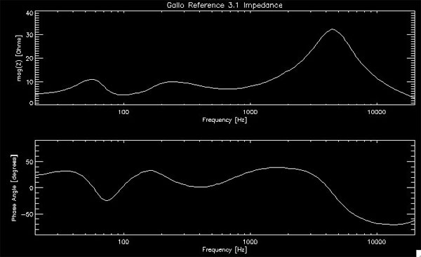
We see that the phase deviates in the capacitive direction quite a lot at high frequencies, and that the real part of the impedance gets very high at about 5 kHz. From rules of thumb, you can say that this speaker should be not too difficult to drive, but things get a little funky towards the high end. Since tweeters consume very little power, this shouldn’t be too big of a deal in terms of taxing the amplifier. Still, this plot is a little difficult to interpret at one glance. The actual load in terms of resistance and reactance is a combination of both plots at the same time. A high or low resistance magnitude is OK as long as it does not also come with a high phase angle. A high phase angle means more resistance or capacitance if the magnitude of the impedance is high at the same time.

What if we plot the same data on the Smith chart? Now we see both the real and imaginary part at the same time. The plot is set to have 8 ohms in the center. A perfect 8 ohm resistive load would be a speck at the center of the plot. Deviation from a perfect 8 ohm load moves the line away from the center of the plot. This plot is relatively easy to interpret. The closer the squiggly line is to the center of the plot, the easier the speaker is to drive. Failing that, it’s better to move along the center-line than deviate a lot above or below.

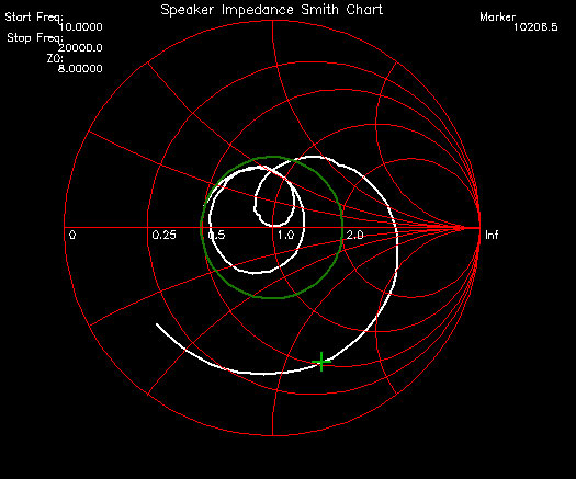
To get back some of the frequency information I’ve put a green marker (+) on the plot, with a frequency of 10.2 kHz corresponding to the marker (10,200 Hz). We can see here that the speaker does well throughout most of its range, but becomes more difficult to drive at one frequency extreme. To tell what frequency extreme requires either the other plotting method, or using a marker as shown. This plot has an adjustable “reference impedance.” Here Z0, the reference impedance, is set to 8 ohms. The center-line of the plot shows the real part of the impedance in fractions of Z0. The center is 1 times Z0, or 8 ohms. 0.5 to the left is 0.5 times Z0, or 4 ohms, 2.0 to the right is 2.0 times Z0 or 16 ohms. For simplicity, I have left off the units for the capacitance and inductance.

Really, the units are not important for using this plot to quickly analyze a speaker load. The main thing is how close to the center of the plot the line is. I would call an “easy load” any impedance that remains inside the green circle on the plot (within a factor of two of 8 ohms). The Gallos do well for most of the range, but the tweeter rapidly runs away in impedance.  This wacky tweeter impedance could be a problem for some electronics, and is probably a result of the “crossoverless” design of the Gallos.

Luckily, a tweeter that presents a difficult load is not that big of a deal. If this same impedance issue were present at the other frequency extreme (low frequencies), there would be a big problem. Engineering an amp capable of driving a woofer with an impedance that crazy would be quite a feat.

Conclusions

While the Smith chart certainly is not the typical way to plot speaker impedance in audio engineering, I believe it does have a place. It makes speaker impedance far easier to interpret at a glance than the normal method using two separate plots, without having to be a speaker guru.